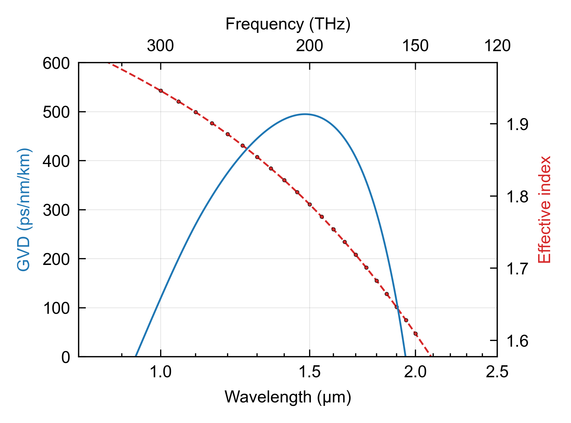
Dispersion Sweep
The sweep function is demonstrated to calculate dispersion of a waveguide. See for a comparison: J. A. Black, R. Streater, K. F. Lamee, D. R. Carlson, S.-P. Yu, and S. B. Papp, “Group-velocity-dispersion engineering of tantala integrated photonics,” Opt. Lett. 46, 817 (2021).
This code example is licensed under the BSD 3-Clause License.
import emodeconnection as emc
import numpy as np

## Set simulation parameters
dx, dy = 10, 10 # [nm] resolution
h_core = 750 # [nm] waveguide core height
b_clad = 2500 # [nm] waveguide top and bottom clad
h_clad = 1500 # [nm] waveguide top and bottom clad
w_core = h_core*1.25 # [nm] waveguide core width
w_trench = 2500 # [nm] waveguide side trench width
num_modes = 1 # [-] number of modes
boundary = 'TE'

wav_nm_ = np.arange(1000, 2001, 50) # [nm]

## Connect and initialize EMode
em = emc.EMode(simulation_name = 'dispersion')

## Settings
em.settings(
    x_resolution = dx, y_resolution = dy,
    window_width = w_core + w_trench*2,
    window_height = h_core + b_clad + h_clad,
    num_modes = num_modes, boundary_condition = boundary,
    background_material = 'Air')

## Draw shapes
em.shape(name = 'BOX', material = 'SiO2', height = b_clad)
em.shape(name = 'core', material = 'Ta2O5', width = w_core,
    height = h_core)

## Run wavelength sweep
data = em.sweep(key = 'wavelength', values = wav_nm_,
    result = ['effective_index'])

## Close EMode
em.close()
Console output:
EMode3D 1.0.1 - email

Sweeping setting parameter 'wavelength'...
Solving FDM: wavelength = 1000... completed in 2.2 sec
Solving FDM: wavelength = 1050... completed in 1.9 sec
Solving FDM: wavelength = 1100... completed in 1.9 sec
Solving FDM: wavelength = 1150... completed in 1.7 sec
Solving FDM: wavelength = 1200... completed in 1.9 sec
Solving FDM: wavelength = 1250... completed in 1.8 sec
Solving FDM: wavelength = 1300... completed in 1.8 sec
Solving FDM: wavelength = 1350... completed in 1.9 sec
Solving FDM: wavelength = 1400... completed in 1.7 sec
Solving FDM: wavelength = 1450... completed in 1.9 sec
Solving FDM: wavelength = 1500... completed in 1.9 sec
Solving FDM: wavelength = 1550... completed in 1.9 sec
Solving FDM: wavelength = 1600... completed in 1.9 sec
Solving FDM: wavelength = 1650... completed in 2.0 sec
Solving FDM: wavelength = 1700... completed in 2.0 sec
Solving FDM: wavelength = 1750... completed in 1.9 sec
Solving FDM: wavelength = 1800... completed in 2.0 sec
Solving FDM: wavelength = 1850... completed in 2.1 sec
Solving FDM: wavelength = 1900... completed in 1.8 sec
Solving FDM: wavelength = 1950... completed in 2.0 sec
Solving FDM: wavelength = 2000... completed in 1.9 sec
 completed in 39.9 sec
Exited EMode
A separate script can be used to plot the results.
import emodeconnection as emc
from emodeconnection import constants
import numpy as np
from scipy.interpolate import UnivariateSpline

## Extract sweep results without an EMode license
data = emc.get(variable = 'sweep_data', simulation_name = 'dispersion')

## Calculate dispersion
ind = np.argsort(data['values'])
n_eff_spl = UnivariateSpline(
    data['values'][ind], data['effective_index'][ind], s=0, k=4)

n_eff_spl_2d = n_eff_spl.derivative(n = 2)
wav_nm_fit = np.arange(800, 2501, 1) # [nm]
D = -wav_nm_fit/constants.c*n_eff_spl_2d(wav_nm_fit)*1e12/1e-3 # [ps/nm/km]

## Plot
import matplotlib.pyplot as plt
from matplotlib import rc as mplrc

fw, LW = 8/2.54, 0.5
mplrc('font',**{'family':'sans-serif','size':7})
mplrc('axes', linewidth=LW, axisbelow=True)
mplrc('xtick', bottom=True, top=True, direction='in')
mplrc('ytick', left=True, right=True, direction='in')
mplrc('xtick.major', size=3, width=LW)
mplrc('xtick.minor', size=1.5, width=LW)
mplrc('ytick.major', size=3, width=LW)
mplrc('figure',figsize=[fw, fw/2**0.5])

fig, ax = plt.subplots(1, 1)
ax.set_xlabel(u'Wavelength (\u03bcm)')
ax.set_ylabel('GVD (ps/nm/km)', color = 'tab:blue')
ax.axes.set_xscale('log')
ax2 = ax.twinx()
ax2.set_ylabel('Effective index', color = 'tab:red')
ax.grid(visible=True, which='major', axis='both', linewidth=LW/2, color='grey', alpha=0.25)

ax.plot(wav_nm_fit, D,
    color = 'tab:blue', marker = '', linestyle = '-',
    lw = LW*1.5)

ax2.plot(wav_nm_fit, n_eff_spl(wav_nm_fit),
    color = 'tab:red', marker = '', linestyle = '--',
    lw = LW*1.5)

ax2.plot(data['values'], data['effective_index'],
    color = 'tab:red', marker = 'o', linestyle = '',
    ms = 1.5, mec = 'k', mew = 0.2)

ax.set_xlim([800, 2500])
xticks_nm = np.array([1000, 1500, 2000, 2500])
xticks_nm_minor = np.arange(800, 2500.1, 100)
ax.set_xticks(xticks_nm_minor, labels=''*len(xticks_nm_minor), minor=True)
ax.set_xticks(xticks_nm)
ax.set_xticklabels(['%0.1f' % (x*1e-3) for x in xticks_nm])
ax.set_ylim([0, 600])
ax2.set_ylim([
    np.min(data['effective_index'])*0.98,
    np.max(data['effective_index'])*1.02])

ax3 = ax.twiny()
ax3.axes.set_xscale('log')
ax3.set_xlim(ax.get_xlim())
ax3.set_xlabel('Frequency (THz)')
ax3.set_xticks(xticks_nm)
ax3.set_xticklabels(['%0.0f' % x for x in constants.c/xticks_nm*1e-3])
ax.set_zorder(ax2.get_zorder()+1)
ax.patch.set_visible(False)

fig.savefig('dispersion.png', dpi = 600, bbox_inches = 'tight')
Figures: