Open a Simulation
How to open an existing EMode simulation.
This code example is licensed under the BSD 3-Clause License.
import emodeconnection as emc
## Run an initial session with a unique simulation name.
# Set simulation parameters
wavelength = 1970 # [nm] wavelength
dx, dy = 10, 5 # [nm] resolution
trench = 1200 # [nm] waveguide side trench width
t_clad = 1200 # [nm] waveguide top/bot clad
b_clad = 1500 # [nm] waveguide top/bot clad
w_core = 1734 # [nm] waveguide core width
h_core = 150 # [nm] waveguide core height
h_slab = 20 # [nm] slab thickness in etched areas
angle = 17 # [degrees] waveguide sidewall angle
width = w_core + trench*2 # [nm] window width
height = h_core + b_clad + t_clad # [nm] window height
num_modes = 1 # [nm] number of modes
boundary = 'TE'
# Connect and initialize EMode
em = emc.EMode(simulation_name = 'GaAs_SHG')
# Settings
em.settings(
wavelength = wavelength,
x_resolution = dx, y_resolution = dy,
window_width = width, window_height = height,
boundary_condition = boundary, num_modes = num_modes,
background_material = "Air")
# Draw shapes
em.shape(name = "BOX", material = "SiO2", height = b_clad)
em.shape(name = "core", material = "GaAs", sidewall_angle = angle,
mask = w_core, height = h_core, etch_depth = h_core - h_slab)
# Launch FDM solver
em.FDM()
em.report()
em.close()
## The previous simulated can be opened again, modified, and saved with a new name.
# Open existing simulation file
em = emc.EMode(simulation_name = 'GaAs_SHG',
open_existing = True, new_name = 'GaAs_SHG-TM')
# Get the previous wavelength setting and convert it to the second harmonic wavelength
wavelength = em.get('wavelength')/2
n_eff = em.get('effective_index')
# Update the settings
em.settings(wavelength = wavelength,
boundary_condition = 'TM', num_modes = 2,
max_effective_index = n_eff[0])
# Launch FDM solver
em.FDM()
em.report()
em.close()
## When opening an existing file to only retrieve and plot data, a new simulation name is not needed since the simulation data will not be modified.
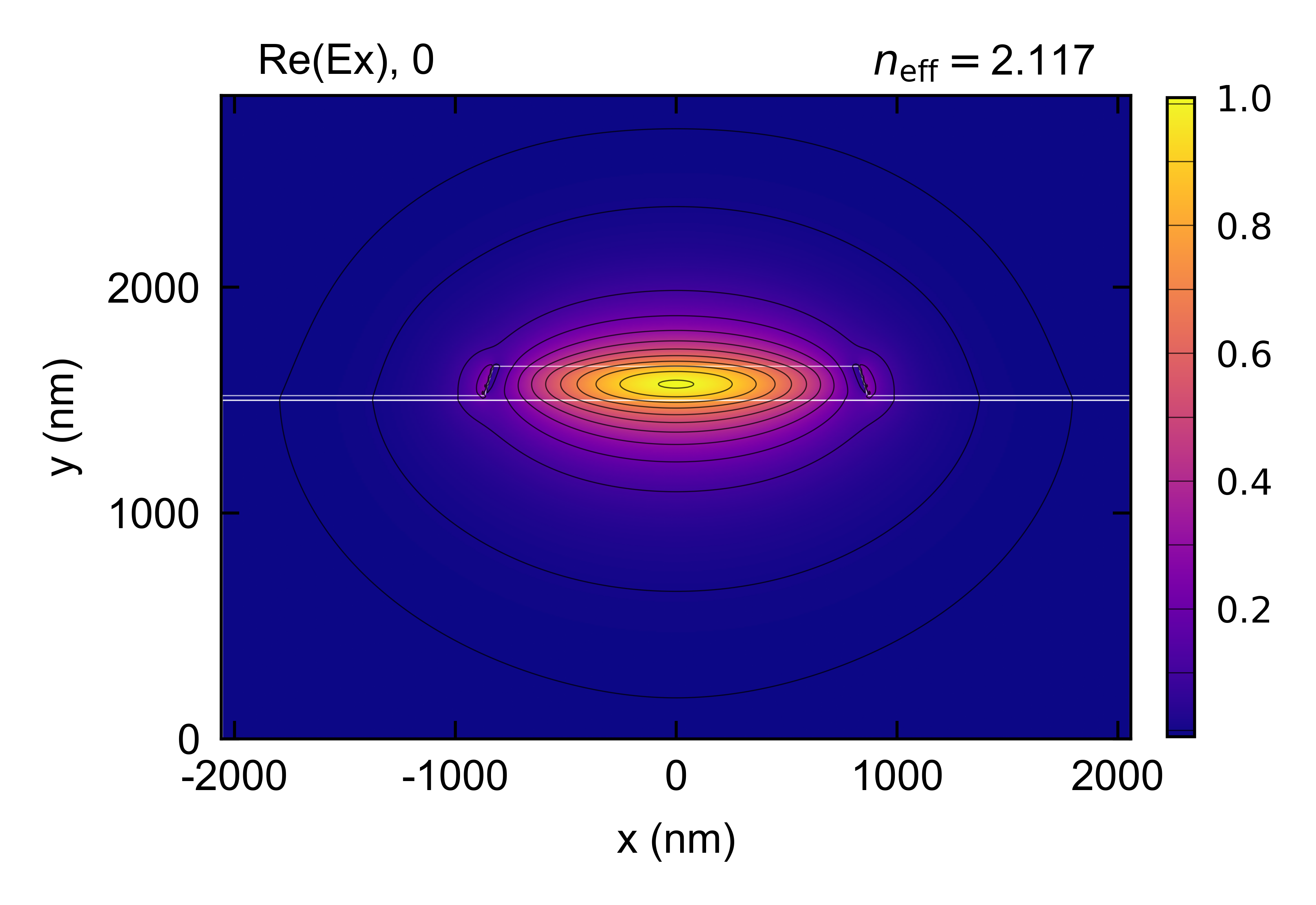
# Plot from existing simulation file - pump mode
em = emc.EMode(simulation_name = 'GaAs_SHG', open_existing = True)
E_p = em.get_fields(key = ['Ex', 'Ey', 'Ez'])
em.plot()
em.close()
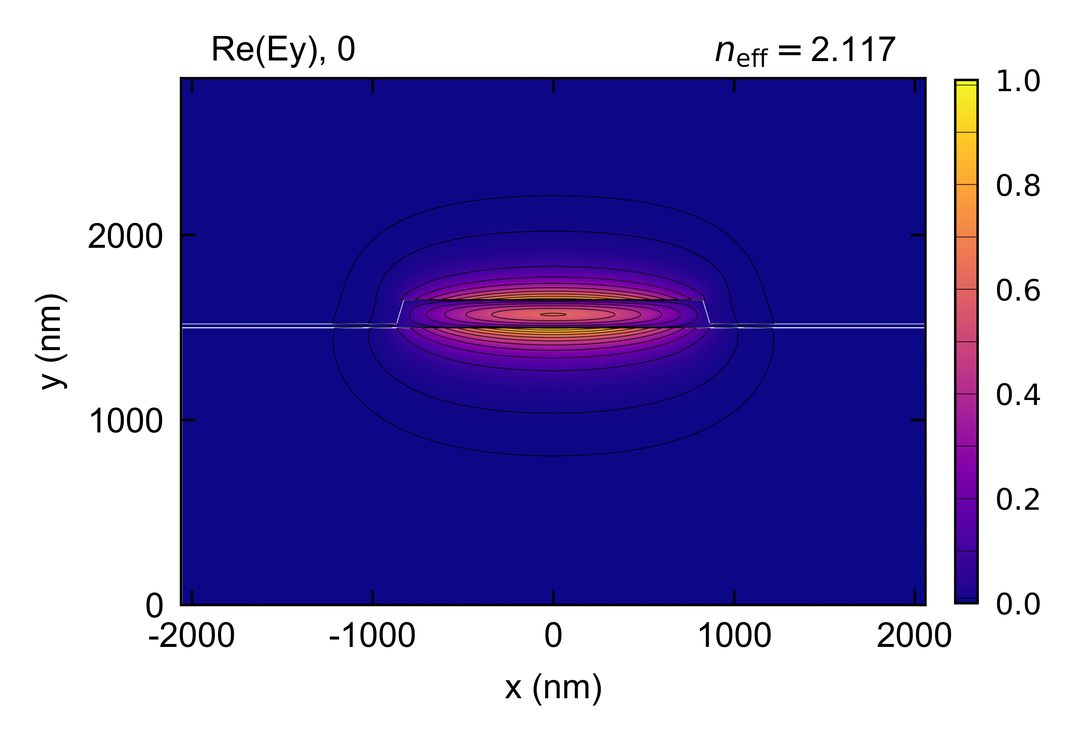
# Plot from existing simulation file - signal mode
em = emc.EMode(simulation_name = 'GaAs_SHG-TM', open_existing = True)
E_s = em.get_fields(key = ['Ex', 'Ey', 'Ez'])
TM_indices = em.get('TM_indices')
em.plot(component = 'Ey', mode = TM_indices[0])
em.close()
Console output:
EMode3D 1.0.1 - email
Meshing completed in 0.7 sec
Solving modes completed in 1.4 sec

Wavelength: 1970.0 nm

  Mode #     n_eff    TE %    Loss (dB/m)
--------  --------  ------  -------------
    TE-0  2.094190  99.8 %          0.000

Exited EMode
EMode3D 1.0.1 - email
Meshing completed in 0.7 sec
Solving modes completed in 1.6 sec

Wavelength: 985.0 nm

  Mode #     n_eff    TE %    Loss (dB/m)
--------  --------  ------  -------------
    TM-0  2.067847   1.2 %          0.000
    TM-1  1.929029  15.3 %          0.000

Exited EMode
EMode3D 1.0.1 - email
Exited EMode
EMode3D 1.0.1 - email
Exited EMode
Figures: