EME: Sweep
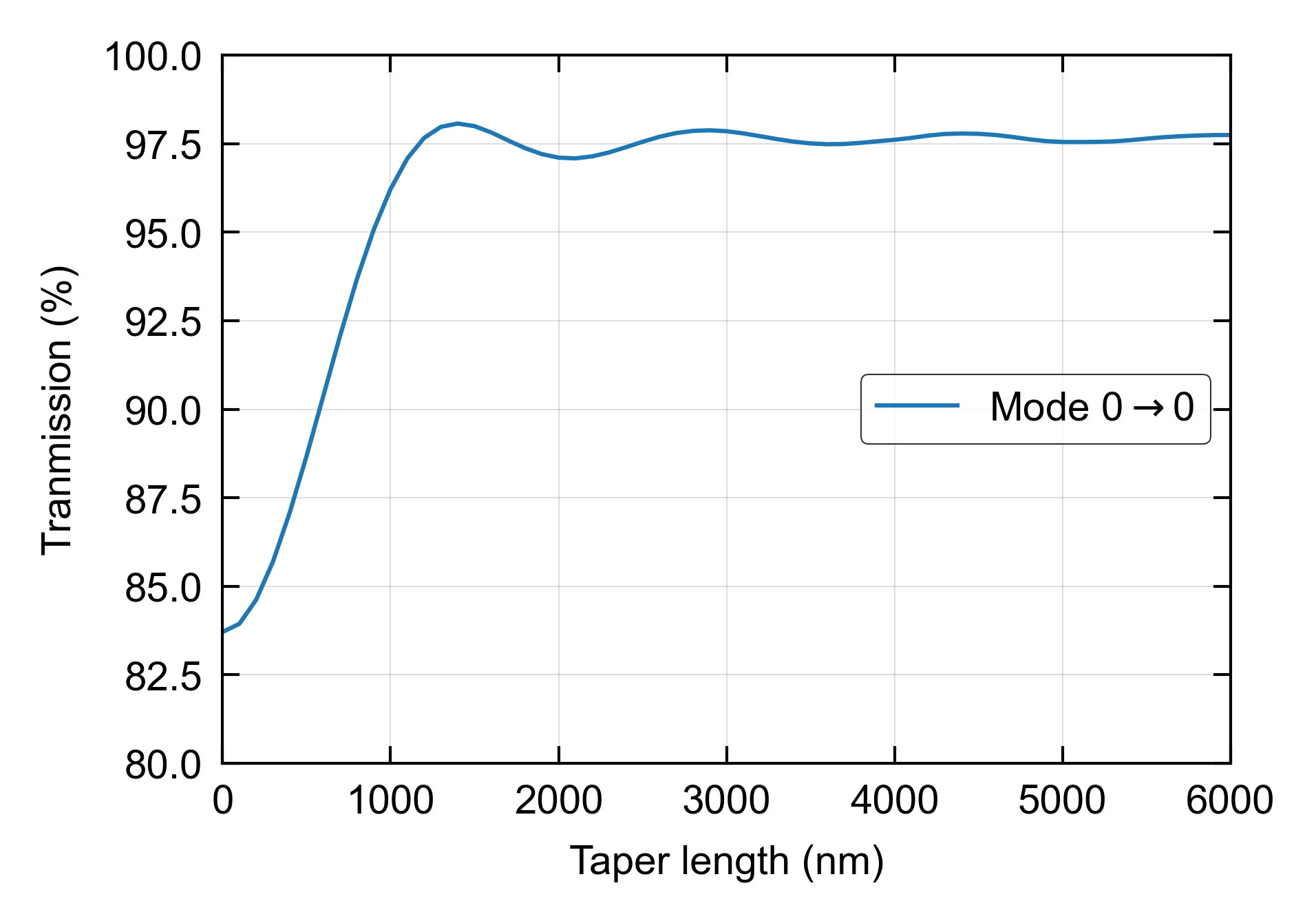
In practice, a taper length needs to be optimized to ensure proper modal transmission and low loss. This example shows how the sweep function can be used to visualize the transmission of an EME taper simulation.
This code example is licensed under the BSD 3-Clause License.
import emodeconnection as emc
import numpy as np

## Set simulation parameters
wavelength = 1550 # [nm] wavelength
dx, dy = 20, 20 # [nm] resolution
h_core = 220 # [nm] waveguide core height
h_clad = 1000 # [nm] waveguide top and bottom clad

window_width = 4000
window_height = h_core + h_clad*2

num_modes = 10 # [-] number of modes
BC = 'TE'

## Connect and initialize EMode
em = emc.EMode(simulation_name = 'taper', verbose = True)

## Settings
em.settings(
    wavelength = wavelength, x_resolution = dx, y_resolution = dy,
    window_width = window_width, window_height = window_height,
    num_modes = num_modes, boundary_condition = BC,
    background_material = 'SiO2')

## Draw shapes
em.shape(name = 'BOX', material = 'SiO2',
    height = h_clad)
em.shape(name = 'core', material = 'Si',
height = h_core, etch_depth = h_core)

## Launch FDM solver and label profiles
em.shape(name = 'core', mask = 1000)
em.label_profile(name = 'a') # skips solving the modes here

em.shape(name = 'core', mask = 2000)
em.label_profile(name = 'b') # skips solving the modes here

## Draw EME sections
em.straight_section(
    profile = 'a',
    length = 2000)

em.taper_section(name = 'taper',
    profile = 'a', profile_end = 'b',
    length = 8000)

em.straight_section(
    profile = 'b',
    length = 2000)

## Run EME sweep
data = em.sweep(key = 'section, taper, length',
    values = np.arange(0, 8001, 250),
    result = ['S_matrix'])

## Close EMode
em.close()
Console output:
EMode3D 1.0.1 - email
Saved profile: 'a'
Saved profile: 'b'

Sweeping section parameter 'length'...
Solving EME: length = 8000...
Solving slice at 4000.0 nm... completed in 0.5 sec
Solving slice at 6000.0 nm... completed in 0.6 sec
Solving slice at 2000.0 nm... completed in 0.5 sec
Solving slice at 7000.0 nm... completed in 0.6 sec
Solving slice at 5000.0 nm... completed in 0.6 sec
Solving slice at 3000.0 nm... completed in 0.6 sec
Solving slice at 1000.0 nm... completed in 0.6 sec
Solving slice at 7500.0 nm... completed in 0.6 sec
Solving slice at 6500.0 nm... completed in 0.5 sec
Solving slice at 5500.0 nm... completed in 0.5 sec
Solving slice at 4500.0 nm... completed in 0.5 sec
Solving slice at 3500.0 nm... completed in 0.5 sec
Solving slice at 2500.0 nm... completed in 0.5 sec
Solving slice at 1500.0 nm... completed in 0.5 sec
Solving slice at 500.0 nm... completed in 0.5 sec
Solving slice at 7750.0 nm... completed in 0.5 sec
Solving slice at 7250.0 nm... completed in 0.5 sec
Solving slice at 6750.0 nm... completed in 0.5 sec
Solving slice at 6250.0 nm... completed in 0.5 sec
Solving slice at 5750.0 nm... completed in 0.5 sec
Solving slice at 5250.0 nm... completed in 0.5 sec
Solving slice at 4750.0 nm... completed in 0.5 sec
Solving slice at 4250.0 nm... completed in 0.5 sec
Solving slice at 3750.0 nm... completed in 0.5 sec
Solving slice at 3250.0 nm... completed in 0.5 sec
Solving slice at 2750.0 nm... completed in 0.5 sec
Solving slice at 2250.0 nm... completed in 0.6 sec
Solving slice at 1750.0 nm... completed in 0.5 sec
Solving slice at 1250.0 nm... completed in 0.5 sec
Solving slice at 750.0 nm... completed in 0.5 sec
Solving slice at 250.0 nm... completed in 0.5 sec
Solving slice at 6125.0 nm... completed in 0.5 sec
Solving slice at 5875.0 nm... completed in 0.5 sec
Solving slice at 5375.0 nm... completed in 0.5 sec
Solving slice at 5125.0 nm... completed in 0.5 sec
Solving slice at 4375.0 nm... completed in 0.6 sec
Solving slice at 4125.0 nm... completed in 0.6 sec
Solving slice at 3875.0 nm... completed in 0.5 sec
Solving slice at 3625.0 nm... completed in 0.5 sec
Solving slice at 3375.0 nm... completed in 0.5 sec
Solving slice at 3125.0 nm... completed in 0.5 sec
Solving slice at 2875.0 nm... completed in 0.5 sec
Solving slice at 2625.0 nm... completed in 0.5 sec
Solving slice at 2375.0 nm... completed in 0.5 sec
Solving slice at 5437.5 nm... completed in 0.5 sec
Solving slice at 5312.5 nm... completed in 0.5 sec
Solving slice at 5187.5 nm... completed in 0.5 sec
Solving slice at 4312.5 nm... completed in 0.5 sec
Solving slice at 4187.5 nm... completed in 0.5 sec
Solving slice at 2562.5 nm... completed in 0.5 sec
Solving slice at 2312.5 nm... completed in 0.5 sec
Solving slice at 4218.8 nm... completed in 0.5 sec
 completed in 37.6 sec
Solving EME: length = 7750... completed in 0.0 sec
Solving EME: length = 7500... completed in 0.0 sec
Solving EME: length = 7250... completed in 0.0 sec
Solving EME: length = 7000... completed in 0.0 sec
Solving EME: length = 6750... completed in 0.0 sec
Solving EME: length = 6500... completed in 0.0 sec
Solving EME: length = 6250... completed in 0.0 sec
Solving EME: length = 6000... completed in 0.0 sec
Solving EME: length = 5750... completed in 0.0 sec
Solving EME: length = 5500... completed in 0.0 sec
Solving EME: length = 5250... completed in 0.0 sec
Solving EME: length = 5000... completed in 0.0 sec
Solving EME: length = 4750... completed in 0.0 sec
Solving EME: length = 4500... completed in 0.0 sec
Solving EME: length = 4250... completed in 0.0 sec
Solving EME: length = 4000... completed in 0.0 sec
Solving EME: length = 3750... completed in 0.0 sec
Solving EME: length = 3500... completed in 0.0 sec
Solving EME: length = 3250... completed in 0.0 sec
Solving EME: length = 3000... completed in 0.0 sec
Solving EME: length = 2750... completed in 0.0 sec
Solving EME: length = 2500... completed in 0.0 sec
Solving EME: length = 2250... completed in 0.0 sec
Solving EME: length = 2000... completed in 0.0 sec
Solving EME: length = 1750... completed in 0.0 sec
Solving EME: length = 1500... completed in 0.0 sec
Solving EME: length = 1250... completed in 0.0 sec
Solving EME: length = 1000... completed in 0.0 sec
Solving EME: length = 750... completed in 0.0 sec
Solving EME: length = 500... completed in 0.0 sec
Solving EME: length = 250... completed in 0.0 sec
Solving EME: length = 0... completed in 0.0 sec
 completed in 38.6 sec
Exited EMode
While no figures are generated in the EMode script, a separate script can be used to plot the results.
import emodeconnection as emc
import numpy as np
## Extract sweep results without an EMode license
data = emc.get(variable = 'sweep_data', simulation_name = 'taper')
## Plot
import matplotlib.pyplot as plt
from matplotlib import rc as mplrc
fw, LW = 8/2.54, 0.5
mplrc('font',**{'family':'sans-serif','size':7})
mplrc('axes', linewidth=LW, axisbelow=True)
mplrc('xtick', bottom=True, top=True, direction='in')
mplrc('ytick', left=True, right=True, direction='in')
mplrc('xtick.major', size=3, width=LW)
mplrc('ytick.major', size=3, width=LW)
mplrc('figure',figsize=[fw, fw/2**0.5])
fig, ax = plt.subplots(1, 1)
ax.set_xlabel('Taper length (nm)')
ax.set_ylabel('Transmission (%)')
ax.grid(visible=True, which='major', axis='both', linewidth=LW/2, color='grey', alpha=0.25)
transmission = np.array([s.transmission() for s in data['S_matrix']])
lines = []
for kk in range(transmission.shape[-1]):
line, = ax.plot(data['values'],
100*np.abs(transmission[:,kk,0])**2,
marker = '', linestyle = '-', lw = LW*1.5,
label = r'Mode 0$\rightarrow$%d' % kk)
lines.append(line)
ax.set_xlim([
np.min(data['values']),
np.max(data['values'])])
lg = ax.legend(handles = lines[0:1], loc = 'center right')
lg.get_frame().set_linewidth(LW/2)
lg.get_frame().set_edgecolor('k')
ax.set_ylim([70, 101])
fig.savefig('taper_1.png', dpi=600, bbox_inches='tight')
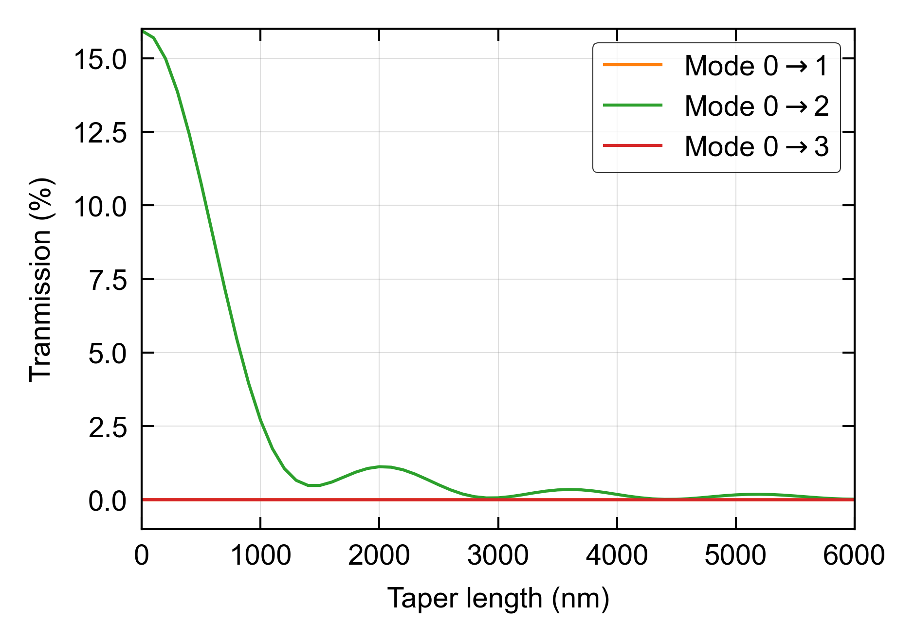
lg = ax.legend(handles = lines[1:10], loc = 'upper right')
lg.get_frame().set_linewidth(LW/2)
lg.get_frame().set_edgecolor('k')
ax.set_ylim([-1, 25])
fig.savefig('taper_2.png', dpi=600, bbox_inches='tight')
Figures: