
Nonlinear-EME: DFG
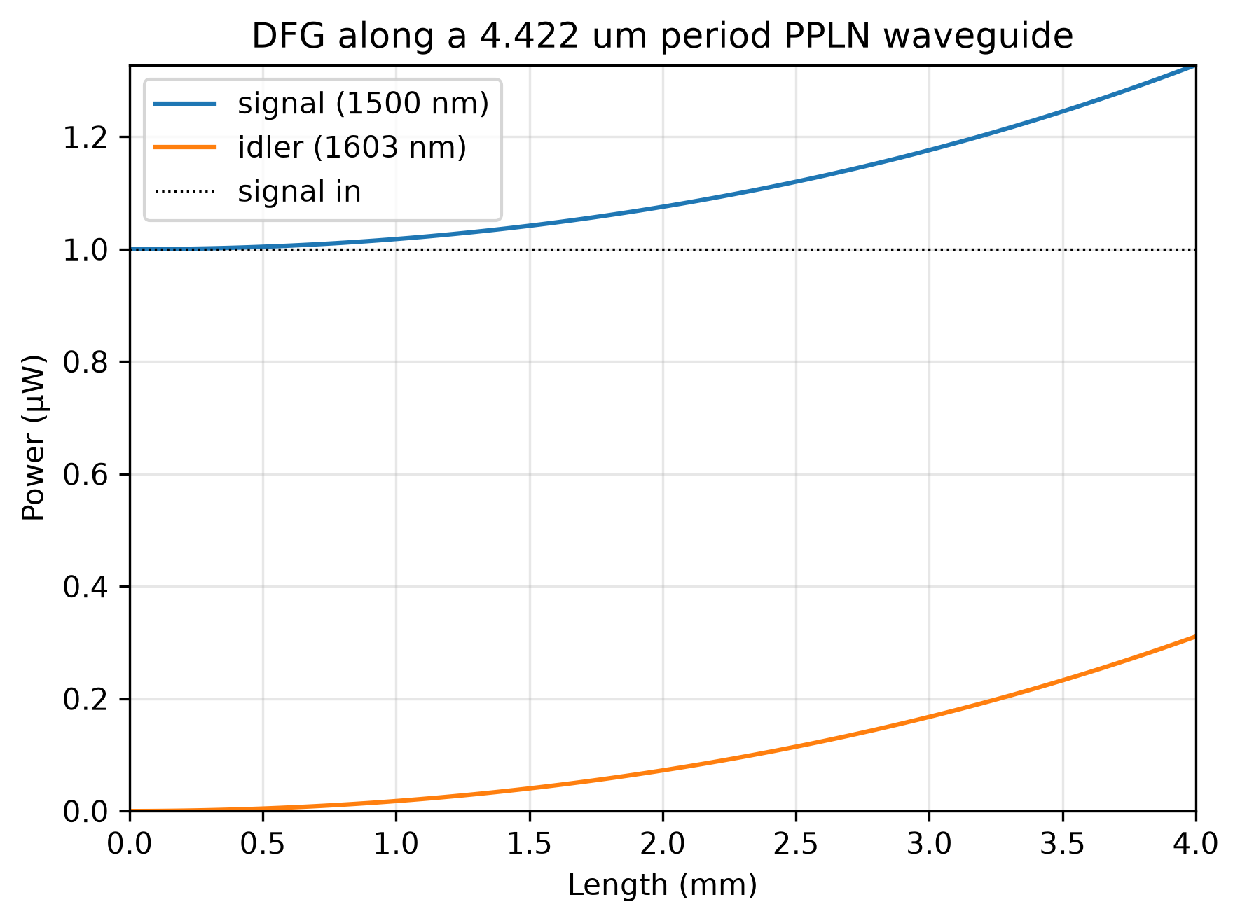
Difference-frequency generation in a periodically poled thin-film lithium niobate waveguide: a 775 nm pump amplifies a 1500 nm signal and builds its 1603 nm idler.
Highlighted features: DFGProcess with poling_period, two simultaneous Source excitations, pml_seed_bool to keep the guided mode at index 0 under a PML, and a three-wavelength profile set.
This code example is licensed under the BSD 3-Clause License.
import sys

import emodeconnection as emc
import numpy as np
from matplotlib import pyplot as plt

## Difference-frequency generation in periodically poled thin-film lithium
## niobate: the 775 nm second harmonic the PPLN example makes, used here to
## amplify a 1500 nm signal and generate its 1603 nm idler. Same x-cut ridge,
## so the interaction is again d33 between TE modes.

## Set simulation parameters
pump_wavelength = 775.0  # [nm] shortest of the three, by energy conservation
signal_wavelength = 1500.0  # [nm]
idler_wavelength = 1 / (1 / pump_wavelength - 1 / signal_wavelength)  # [nm]
dx, dy = 20, 20  # [nm] resolution
w_core = 1600  # [nm] ridge top width
h_film, h_ridge = 600, 300  # [nm] LN film thickness and etch depth
h_box, h_clad = 2000, 1000  # [nm] SiO2 below and above
length = 4e6  # [nm] 4 mm
pump_power = 50e-3  # [W]
signal_power = 1e-6  # [W] small enough to leave the pump undepleted

sidewall_angle = 15  # [deg] from vertical
roughness_rms = [2.0, 0.25]  # [nm] rms, [sidewall, top/bottom]
correlation_length = [50.0, 80.0]  # [nm], [sidewall, top/bottom]

window_width = w_core + 2 * 3000
window_height = h_box + h_film + h_clad

## theta = pi/2 puts the optic axis along simulation x: x-cut.
ln_x_cut = emc.MaterialSpec(material='LN_MgO', theta=np.pi / 2)

em = emc.EMode(emode_cmd=sys.argv[1:], simulation_name='dfg')
em.EME_settings(apply_scattering=True)


def build_profile(wavelength, num_modes, name):
    """One TE profile of the poled ridge at a given wavelength."""
    em.settings(
        wavelength=wavelength,
        x_resolution=dx,
        y_resolution=dy,
        window_width=window_width,
        window_height=window_height,
        num_modes=num_modes,
        boundary_condition='TE',
        background_material='SiO2',
        generate_chi2=True,
        ## The idler is the least confined of the three, so the sides absorb its
        ## lateral radiation. A PML needs both companions here: without
        ## pml_seed_bool a PML mode outranks the guided one and Source launches
        ## into the wrong mode, and without remove_pml_modes_bool the absorber's
        ## modes stay in the basis the coupled-mode ODE integrates, where their
        ## large imaginary beta makes it stiff and the solve crawls.
        pml_NSEW_bool=[False, False, True, True],
        pml_seed_bool=True,
        remove_pml_modes_bool=True,
    )
    em.shape(name='BOX', material='SiO2', height=h_box)
    em.shape(
        name='LN',
        material=ln_x_cut,
        fill_material='SiO2',
        height=h_film,
        mask=w_core,
        etch_depth=h_ridge,
        sidewall_angle=sidewall_angle,
        roughness_rms=roughness_rms,
        correlation_length=correlation_length,
    )
    em.shape(name='clad', material='SiO2', height=h_clad)
    em.FDM(scattering=True)
    em.label_profile(name=name)


build_profile(pump_wavelength, 2, 'pump')
## create_profile_set() consumes its profiles; keep a copy to plot at the end.
em.label_profile(name='pump_mode')
build_profile(signal_wavelength, 1, 'signal')
build_profile(idler_wavelength, 1, 'idler')

def fundamental_te(profile):
    """Index and effective index of the highest-index genuinely TE mode.

    Eigenvalue order is not polarization order: at 775 nm a TM mode sits at
    index 0 even under a TE boundary condition. Launching the pump into it asks
    d33 for an interaction it does not have and the idler comes out at zero.
    """
    n_eff = np.real(np.asarray(em.get('effective_index', profile=profile)))
    te = np.asarray(em.get('TE_fraction', profile=profile))
    index = next(i for i in range(len(n_eff)) if te[i] > 0.5)
    return index, n_eff[index]


## Read the profiles before create_profile_set() consumes them.
i_pump, n_pump = fundamental_te('pump')
i_signal, n_signal = fundamental_te('signal')
i_idler, n_idler = fundamental_te('idler')
for label, wl, i, n in (
    ('pump  ', pump_wavelength, i_pump, n_pump),
    ('signal', signal_wavelength, i_signal, n_signal),
    ('idler ', idler_wavelength, i_idler, n_idler),
):
    print(f'{label} {wl:8.2f} nm: mode {i}, n_eff {n:.5f}')

em.create_profile_set(profiles=['pump', 'signal', 'idler'], profile_set_name='wg')

## Quasi-phase matching cancels what is left: Lambda = 2*pi/Delta_beta, with
## Delta_beta = beta_pump - beta_signal - beta_idler.
delta_beta = 2 * np.pi * (
    n_pump / pump_wavelength - n_signal / signal_wavelength - n_idler / idler_wavelength
) * 1e9
poling_period = 2 * np.pi / delta_beta * 1e9  # [nm]
print(f'poling period: {poling_period * 1e-3:.4f} um')

process = emc.DFGProcess(
    pump_wavelength=pump_wavelength,
    signal_wavelength=signal_wavelength,
    poling_period=poling_period,
)
sources = [
    emc.Source(port='left', wavelength=pump_wavelength, power=pump_power, mode=i_pump),
    emc.Source(port='left', wavelength=signal_wavelength, power=signal_power, mode=i_signal),
]

## Growth along the device. The signal is amplified and the idler built from
## nothing, each pump photon splitting into one of each.
em.straight_section(name='dfg_section', profile='wg', length=length, nonlinear=process)
em.settings(excitation=sources)

em.EME()
r = em.get('response')

## One solve is the whole length scan. The coupled-amplitude solver integrates
## along z anyway, so power_vs_z reads its trajectory back rather than re-solving
## the EME once per length, and all three waves come off the same integration.
z_nm, p_signal = r.power_vs_z(signal_wavelength)
_, p_idler = r.power_vs_z(idler_wavelength)
_, p_pump = r.power_vs_z(pump_wavelength)

gain_dB = 10 * np.log10(p_signal / signal_power)
print(f'signal gain at {length * 1e-6:.0f} mm: {gain_dB[-1]:.3f} dB')
print(f'idler at {length * 1e-6:.0f} mm: {p_idler[-1] * 1e6:.4f} uW')
print(f'pump depletion: {(pump_power - p_pump[-1]) / pump_power * 100:.3f} %')

## Manley-Rowe: every signal photon gained is one idler photon created. Photon
## flux goes as P*lambda, so the ratio is 1 when the bookkeeping is right.
photons_signal = (p_signal[-1] - signal_power) * signal_wavelength
photons_idler = p_idler[-1] * idler_wavelength
print(f'Manley-Rowe (signal gained / idler created): {photons_signal / photons_idler:.4f}')

plt.figure(figsize=(6, 4.5))
plt.plot(z_nm * 1e-6, p_signal * 1e6, label=f'signal ({signal_wavelength:.0f} nm)')
plt.plot(z_nm * 1e-6, p_idler * 1e6, label=f'idler ({idler_wavelength:.0f} nm)')
plt.axhline(signal_power * 1e6, color='k', lw=0.8, ls=':', label='signal in')
plt.xlabel('Length (mm)')
plt.ylabel('Power (\u03BCW)')
plt.title(f'DFG along a {poling_period * 1e-3:.3f} um period PPLN waveguide')
plt.legend()
plt.grid(True, alpha=0.3)
plt.margins(x=0, y=0)
plt.tight_layout()
plt.savefig('dfg_vs_length.png', dpi=300, bbox_inches='tight')

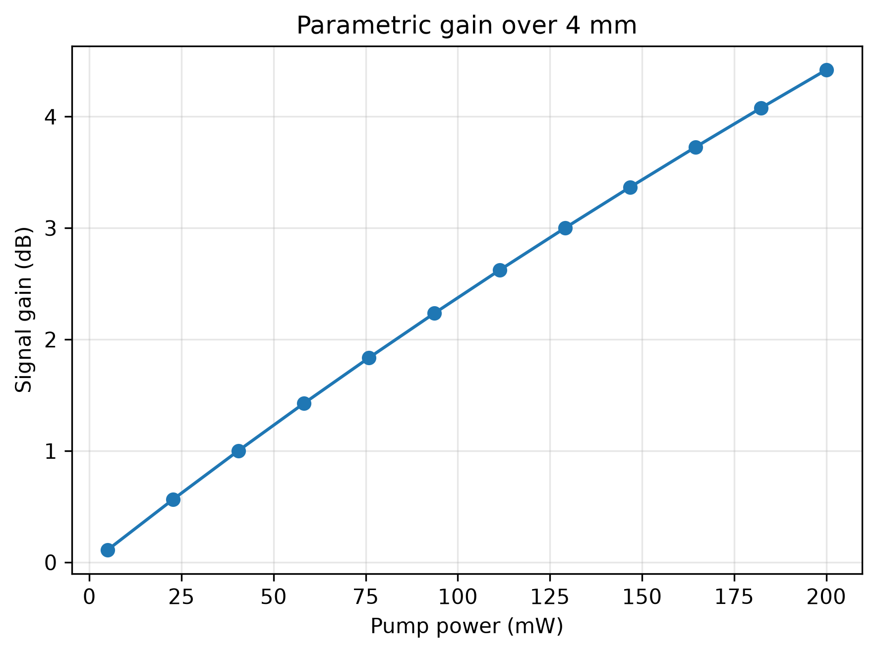
## Gain against pump power. Parametric gain goes as cosh^2(g*L) with g
## proportional to the pump amplitude, so it leaves the quadratic low-gain
## regime and turns exponential once g*L approaches 1. The section is still
## declared at its full length, so only the excitation moves.
pump_powers = np.linspace(5e-3, 200e-3, 12)  # [W]
gain_vs_pump = []
for p in pump_powers:
    em.settings(excitation=[
        emc.Source(port='left', wavelength=pump_wavelength, power=float(p), mode=i_pump),
        emc.Source(port='left', wavelength=signal_wavelength, power=signal_power, mode=i_signal),
    ])
    em.EME()
    r = em.get('response')
    gain_vs_pump.append(r.power('right', signal_wavelength) / signal_power)

plt.figure(figsize=(6, 4.5))
plt.plot(pump_powers * 1e3, 10 * np.log10(gain_vs_pump), marker='o')
plt.xlabel('Pump power (mW)')
plt.ylabel('Signal gain (dB)')
plt.title(f'Parametric gain over {length * 1e-6:.0f} mm')
plt.grid(True, alpha=0.3)
plt.tight_layout()
plt.savefig('dfg_gain_vs_pump.png', dpi=300, bbox_inches='tight')

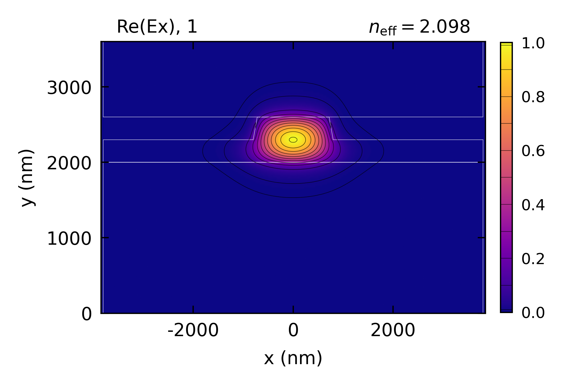
## Mode i_pump, not mode 0: at 775 nm a TM mode sits at index 0 even under a TE
## boundary condition. The same index is declared for dfg_pump_Ex in figures.toml.
em.plot(component='Ex', plot_function='abs', profile='pump_mode', mode=i_pump)

## Close EMode
em.close()
Console output:
EMode3D 1.0.6 - email
Meshing completed in 1.7 sec
Solving modes completed in 4.6 sec
Meshing completed in 1.7 sec
Solving modes completed in 3.9 sec
Meshing completed in 1.7 sec
Solving modes completed in 4.3 sec

Solving S-matrices...
Solving section: dfg_section... completed in 0.4 sec
 completed in 0.4 sec

Solving S-matrices...
Solving section: dfg_section... completed in 0.0 sec
 completed in 0.0 sec

Solving S-matrices...
Solving section: dfg_section... completed in 0.0 sec
 completed in 0.0 sec

Solving S-matrices...
Solving section: dfg_section... completed in 0.0 sec
 completed in 0.0 sec

Solving S-matrices...
Solving section: dfg_section... completed in 0.0 sec
 completed in 0.0 sec

Solving S-matrices...
Solving section: dfg_section... completed in 0.0 sec
 completed in 0.0 sec

Solving S-matrices...
Solving section: dfg_section... completed in 0.0 sec
 completed in 0.0 sec

Solving S-matrices...
Solving section: dfg_section... completed in 0.0 sec
 completed in 0.0 sec

Solving S-matrices...
Solving section: dfg_section... completed in 0.0 sec
 completed in 0.0 sec

Solving S-matrices...
Solving section: dfg_section... completed in 0.0 sec
 completed in 0.0 sec

Solving S-matrices...
Solving section: dfg_section... completed in 0.0 sec
 completed in 0.0 sec

Solving S-matrices...
Solving section: dfg_section... completed in 0.0 sec
 completed in 0.0 sec

Solving S-matrices...
Solving section: dfg_section... completed in 0.0 sec
 completed in 0.0 sec
Exited EMode
pump     775.00 nm: mode 1, n_eff 2.09800
signal  1500.00 nm: mode 0, n_eff 1.93330
idler   1603.45 nm: mode 0, n_eff 1.91144
poling period: 4.4218 um
signal gain at 4 mm: 1.232 dB
idler at 4 mm: 0.3107 uW
pump depletion: 0.946 %
Manley-Rowe (signal gained / idler created): 0.9875
Figures: